> ## Documentation Index
> Fetch the complete documentation index at: https://docs.risingwave.com/llms.txt
> Use this file to discover all available pages before exploring further.
# Server performance anomaly detection
> Detecting performance anomalies in a large fleet of servers and responding as soon as possible has been a challenge for DevOps teams.
## Overview
They set up various metrics to monitor server performance, yet diagnosing performance issues is complex and time-consuming, as the volume of diagnostic data can be huge. There is a growing consensus that it should be automated. But how?
A streaming system can be beneficial in this scenario. It monitors metric performance events in real time right after these events are received and instantly detects anomalies based on patterns defined in SQL queries. Once a performance issue is detected, a downstream micro-service can trigger an action to handle the issue.
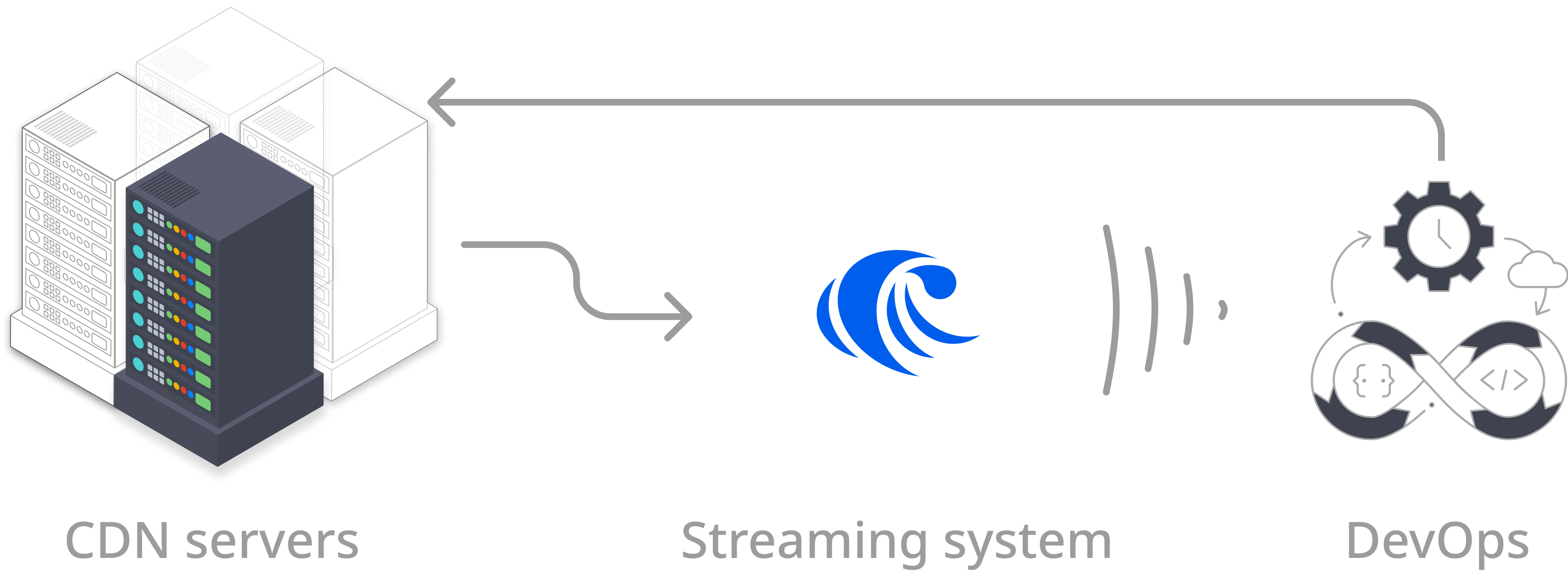 In this tutorial, you will learn how to automate anomaly detection from streams of system performance metrics with RisingWave. We have set up a demo cluster for this tutorial, so you can easily try it out.
## Prerequisites
* Ensure you have [Docker](https://docs.docker.com/get-docker/) and [Docker Compose](https://docs.docker.com/compose/install/) installed in your environment. Note that Docker Compose is included in Docker Desktop for Windows and macOS. If you use Docker Desktop, ensure that it is running before launching the demo cluster.
* Ensure that the [PostgreSQL](https://www.postgresql.org/docs/current/app-psql.html) interactive terminal, `psql`, is installed in your environment. For detailed instructions, see [Download PostgreSQL](https://www.postgresql.org/download/).
## Step 1: Launch the demo cluster
In the demo cluster, we packaged RisingWave and a workload generator. The workload generator will start to generate random traffic and feed them into Kafka as soon as the cluster is started.
First, clone the [risingwave](https://github.com/risingwavelabs/risingwave) repository to the environment.
```bash theme={null}
git clone https://github.com/risingwavelabs/risingwave.git
```
Now navigate to the `integration_tests/cdn-metrics` directory and start the demo cluster from the docker compose file.
```bash theme={null}
cd risingwave/integration_tests/cdn-metrics
docker compose up -d
```
**COMMAND NOT FOUND?**
The default command-line syntax in Compose V2 starts with `docker compose`. See details in the [Docker docs](https://docs.docker.com/compose/migrate/#what-are-the-differences-between-compose-v1-and-compose-v2).
If you're using Compose V1, use `docker-compose` instead.
Necessary RisingWave components will be started, including the Streaming Node, Meta Node, and MinIO. The workload generator will start to generate random data and feed them into Kafka topics. In this demo cluster, data of materialized views will be stored in the MinIO instance.
## Step 2: Connect RisingWave to data streams
Now let's connect to RisingWave so that we can manage data streams and perform data analysis.
```bash theme={null}
psql -h localhost -p 4566 -d dev -U root
```
Now create two separate sources. The first is to track the metrics of network interface cards (NICs), and the second is the metrics stream that tracks the transmission control protocol's (TCP) performance.
```sql theme={null}
CREATE SOURCE nics_metrics (
device_id VARCHAR,
metric_name VARCHAR,
aggregation VARCHAR,
nic_name VARCHAR,
report_time TIMESTAMP WITH TIME ZONE,
bandwidth DOUBLE PRECISION,
metric_value DOUBLE PRECISION
) WITH (
connector = 'kafka',
topic = 'nics_metrics',
properties.bootstrap.server = 'message_queue:29092',
scan.startup.mode = 'earliest'
) FORMAT PLAIN ENCODE JSON;
```
```sql theme={null}
CREATE SOURCE tcp_metrics (
device_id VARCHAR,
metric_name VARCHAR,
report_time TIMESTAMP WITH TIME ZONE,
metric_value DOUBLE PRECISION
) WITH (
connector = 'kafka',
topic = 'tcp_metrics',
properties.bootstrap.server = 'message_queue:29092',
scan.startup.mode = 'earliest'
) FORMAT PLAIN ENCODE JSON;
```
## Step 3: Define materialized views and query the results
In this tutorial, we will create a few different materialized views. The first view, `high_util_tcp_metrics`, will include average values for all metrics of every device every 3 minutes. The other three views will be derived from the first view, each containing a trigger time and different metric values.
### Set up materialized view for highly utilized TCP metrics
First, we will create the materialized view that contains all relevant TCP values. We use the tumble function to map all events into 1-minute windows and calculate the average metric value for each device within each time window. Next, the average TCP and NIC metrics are calculated separately before joining on device names and time windows. We will keep the records measuring the volume of bytes transferred by the interface and where the average utilization is greater than or equal to 50.
Please refer to this [guide](/processing/sql/time-windows) for an explanation of the tumble function and aggregations.
```sql theme={null}
CREATE MATERIALIZED VIEW high_util_tcp_metrics AS
SELECT
tcp.device_id AS device_id,
tcp.window_end AS window_end,
tcp.metric_name AS metric_name,
tcp.metric_value AS metric_value,
nic.avg_util AS tcp_avg_bandwidth_util
FROM
(
SELECT
device_id,
window_end,
metric_name,
AVG(metric_value) AS metric_value
FROM
TUMBLE(
tcp_metrics,
report_time,
INTERVAL '1' MINUTE
)
GROUP BY
device_id,
window_end,
metric_name
) AS tcp
JOIN (
SELECT
device_id,
window_end,
AVG((metric_value) / bandwidth) * 100 AS avg_util
FROM
TUMBLE(
nics_metrics,
report_time,
INTERVAL '1' MINUTE
)
WHERE
metric_name = 'tx_bytes'
AND aggregation = 'avg'
GROUP BY
device_id,
window_end
) AS nic ON tcp.device_id = nic.device_id
AND tcp.window_end = nic.window_end
WHERE
avg_util >= 50;
```
We can see an example of the resulting view by querying the view we just created:
```sql theme={null}
SELECT * FROM high_util_tcp_metrics;
```
Here is an example result.
```bash theme={null}
device_id | window_end | metric_name | metrics_value | tcp_avg_bandwidth_util
----------------------------------+---------------------------+----------------+---------------+-----------------------
eccbc87e4b5ce2fe28308fd9f2a7baf3 | 2022-08-17 18:02:00+00:00 | download_speed | 1126.3827 | 45.26712
eccbc87e4b5ce2fe28308fd9f2a7baf3 | 2022-08-17 18:02:00+00:00 | retrans_rate | 0.19406 | 45.26712
eccbc87e4b5ce2fe28308fd9f2a7baf3 | 2022-08-17 18:02:00+00:00 | srtt | 649.25184 | 45.26712
```
### Set up materialized views from a materialized view
RisingWave supports creating materialized views based on materialized views. Materialized views used as the source are the upstream materialized views, while the materialized views created based on other materialized views are downstream materialized views. As the values of upstream materialized views change, downstream materialized views will change automatically.
In this tutorial, you will learn how to automate anomaly detection from streams of system performance metrics with RisingWave. We have set up a demo cluster for this tutorial, so you can easily try it out.
## Prerequisites
* Ensure you have [Docker](https://docs.docker.com/get-docker/) and [Docker Compose](https://docs.docker.com/compose/install/) installed in your environment. Note that Docker Compose is included in Docker Desktop for Windows and macOS. If you use Docker Desktop, ensure that it is running before launching the demo cluster.
* Ensure that the [PostgreSQL](https://www.postgresql.org/docs/current/app-psql.html) interactive terminal, `psql`, is installed in your environment. For detailed instructions, see [Download PostgreSQL](https://www.postgresql.org/download/).
## Step 1: Launch the demo cluster
In the demo cluster, we packaged RisingWave and a workload generator. The workload generator will start to generate random traffic and feed them into Kafka as soon as the cluster is started.
First, clone the [risingwave](https://github.com/risingwavelabs/risingwave) repository to the environment.
```bash theme={null}
git clone https://github.com/risingwavelabs/risingwave.git
```
Now navigate to the `integration_tests/cdn-metrics` directory and start the demo cluster from the docker compose file.
```bash theme={null}
cd risingwave/integration_tests/cdn-metrics
docker compose up -d
```
**COMMAND NOT FOUND?**
The default command-line syntax in Compose V2 starts with `docker compose`. See details in the [Docker docs](https://docs.docker.com/compose/migrate/#what-are-the-differences-between-compose-v1-and-compose-v2).
If you're using Compose V1, use `docker-compose` instead.
Necessary RisingWave components will be started, including the Streaming Node, Meta Node, and MinIO. The workload generator will start to generate random data and feed them into Kafka topics. In this demo cluster, data of materialized views will be stored in the MinIO instance.
## Step 2: Connect RisingWave to data streams
Now let's connect to RisingWave so that we can manage data streams and perform data analysis.
```bash theme={null}
psql -h localhost -p 4566 -d dev -U root
```
Now create two separate sources. The first is to track the metrics of network interface cards (NICs), and the second is the metrics stream that tracks the transmission control protocol's (TCP) performance.
```sql theme={null}
CREATE SOURCE nics_metrics (
device_id VARCHAR,
metric_name VARCHAR,
aggregation VARCHAR,
nic_name VARCHAR,
report_time TIMESTAMP WITH TIME ZONE,
bandwidth DOUBLE PRECISION,
metric_value DOUBLE PRECISION
) WITH (
connector = 'kafka',
topic = 'nics_metrics',
properties.bootstrap.server = 'message_queue:29092',
scan.startup.mode = 'earliest'
) FORMAT PLAIN ENCODE JSON;
```
```sql theme={null}
CREATE SOURCE tcp_metrics (
device_id VARCHAR,
metric_name VARCHAR,
report_time TIMESTAMP WITH TIME ZONE,
metric_value DOUBLE PRECISION
) WITH (
connector = 'kafka',
topic = 'tcp_metrics',
properties.bootstrap.server = 'message_queue:29092',
scan.startup.mode = 'earliest'
) FORMAT PLAIN ENCODE JSON;
```
## Step 3: Define materialized views and query the results
In this tutorial, we will create a few different materialized views. The first view, `high_util_tcp_metrics`, will include average values for all metrics of every device every 3 minutes. The other three views will be derived from the first view, each containing a trigger time and different metric values.
### Set up materialized view for highly utilized TCP metrics
First, we will create the materialized view that contains all relevant TCP values. We use the tumble function to map all events into 1-minute windows and calculate the average metric value for each device within each time window. Next, the average TCP and NIC metrics are calculated separately before joining on device names and time windows. We will keep the records measuring the volume of bytes transferred by the interface and where the average utilization is greater than or equal to 50.
Please refer to this [guide](/processing/sql/time-windows) for an explanation of the tumble function and aggregations.
```sql theme={null}
CREATE MATERIALIZED VIEW high_util_tcp_metrics AS
SELECT
tcp.device_id AS device_id,
tcp.window_end AS window_end,
tcp.metric_name AS metric_name,
tcp.metric_value AS metric_value,
nic.avg_util AS tcp_avg_bandwidth_util
FROM
(
SELECT
device_id,
window_end,
metric_name,
AVG(metric_value) AS metric_value
FROM
TUMBLE(
tcp_metrics,
report_time,
INTERVAL '1' MINUTE
)
GROUP BY
device_id,
window_end,
metric_name
) AS tcp
JOIN (
SELECT
device_id,
window_end,
AVG((metric_value) / bandwidth) * 100 AS avg_util
FROM
TUMBLE(
nics_metrics,
report_time,
INTERVAL '1' MINUTE
)
WHERE
metric_name = 'tx_bytes'
AND aggregation = 'avg'
GROUP BY
device_id,
window_end
) AS nic ON tcp.device_id = nic.device_id
AND tcp.window_end = nic.window_end
WHERE
avg_util >= 50;
```
We can see an example of the resulting view by querying the view we just created:
```sql theme={null}
SELECT * FROM high_util_tcp_metrics;
```
Here is an example result.
```bash theme={null}
device_id | window_end | metric_name | metrics_value | tcp_avg_bandwidth_util
----------------------------------+---------------------------+----------------+---------------+-----------------------
eccbc87e4b5ce2fe28308fd9f2a7baf3 | 2022-08-17 18:02:00+00:00 | download_speed | 1126.3827 | 45.26712
eccbc87e4b5ce2fe28308fd9f2a7baf3 | 2022-08-17 18:02:00+00:00 | retrans_rate | 0.19406 | 45.26712
eccbc87e4b5ce2fe28308fd9f2a7baf3 | 2022-08-17 18:02:00+00:00 | srtt | 649.25184 | 45.26712
```
### Set up materialized views from a materialized view
RisingWave supports creating materialized views based on materialized views. Materialized views used as the source are the upstream materialized views, while the materialized views created based on other materialized views are downstream materialized views. As the values of upstream materialized views change, downstream materialized views will change automatically.
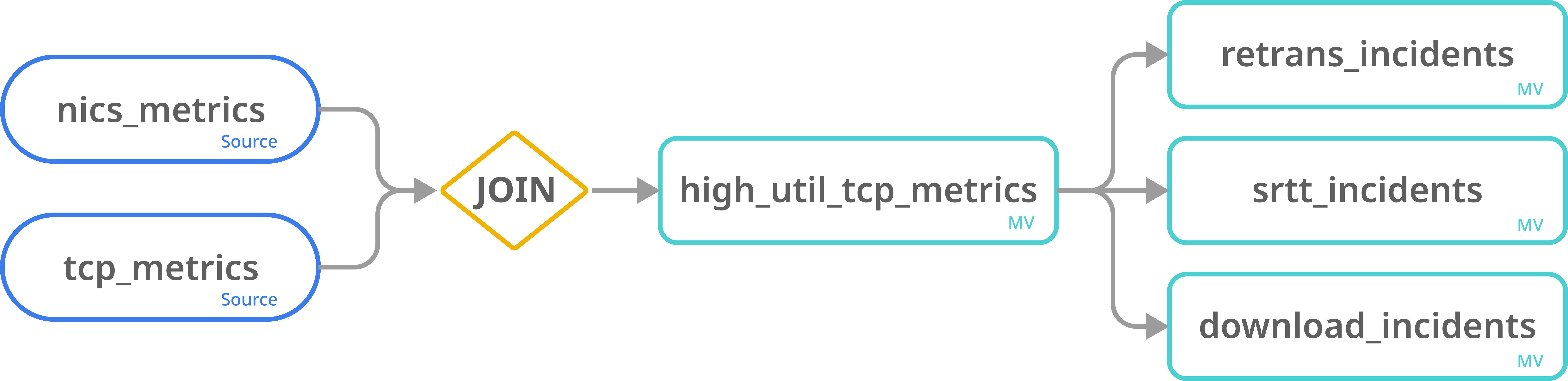 The following three materialized views use high\_util\_tcp\_metrics as their source. The resulting materialized views include detected anomalies of different incidents. An anomaly is detected when the corresponding metric value for an incident is above or below a specific threshold.
The first materialized view queries retransmission timeouts.
```sql theme={null}
CREATE MATERIALIZED VIEW retrans_incidents AS
SELECT
device_id,
window_end AS trigger_time,
metric_value AS trigger_value
FROM
high_util_tcp_metrics
WHERE
metric_name = 'retrans_rate'
AND metric_value > 0.15;
```
The second materialized view queries slow round trip times.
```sql theme={null}
CREATE MATERIALIZED VIEW srtt_incidents AS
SELECT
device_id,
window_end AS trigger_time,
metric_value AS trigger_value
FROM
high_util_tcp_metrics
WHERE
metric_name = 'srtt'
AND metric_value > 500.0;
```
The last materialized view queries download incidents.
```sql theme={null}
CREATE MATERIALIZED VIEW download_incidents AS
SELECT
device_id,
window_end AS trigger_time,
metric_value AS trigger_value
FROM
high_util_tcp_metrics
WHERE
metric_name = 'download_speed'
AND metric_value < 200.0;
```
Now we can display the anomalies detected. We will show `srtt_incidents` as an example, but you can query the other two materialized views. Note that your results will differ because the workload generator randomly generates the data in the streams.
```sql theme={null}
SELECT * FROM srtt_incidents;
```
```bash theme={null}
device_id | trigger_time | trigger_value
---------------------------------+---------------------------+---------------
cfcd208495d565ef66e7dff9f98764da | 2022-08-18 18:02:00+00:00 | 698.14387
e4da3b7fbbce2345d7772b0674a318d5 | 2022-08-18 18:09:00+00:00 | 973.03618
```
You can rerun the query a couple of minutes later to see if the results are updated.
When you finish, run the following command to disconnect RisingWave.
```
\q
```
Optional: To remove the containers and the data generated, use the following command.
```bash theme={null}
docker compose down -v
```
## Summary
In this tutorial, we learn:
* How to set up a streaming pipeline for anomaly detection using RisingWave.
* How to create materialized views based on existing materialized views.
The following three materialized views use high\_util\_tcp\_metrics as their source. The resulting materialized views include detected anomalies of different incidents. An anomaly is detected when the corresponding metric value for an incident is above or below a specific threshold.
The first materialized view queries retransmission timeouts.
```sql theme={null}
CREATE MATERIALIZED VIEW retrans_incidents AS
SELECT
device_id,
window_end AS trigger_time,
metric_value AS trigger_value
FROM
high_util_tcp_metrics
WHERE
metric_name = 'retrans_rate'
AND metric_value > 0.15;
```
The second materialized view queries slow round trip times.
```sql theme={null}
CREATE MATERIALIZED VIEW srtt_incidents AS
SELECT
device_id,
window_end AS trigger_time,
metric_value AS trigger_value
FROM
high_util_tcp_metrics
WHERE
metric_name = 'srtt'
AND metric_value > 500.0;
```
The last materialized view queries download incidents.
```sql theme={null}
CREATE MATERIALIZED VIEW download_incidents AS
SELECT
device_id,
window_end AS trigger_time,
metric_value AS trigger_value
FROM
high_util_tcp_metrics
WHERE
metric_name = 'download_speed'
AND metric_value < 200.0;
```
Now we can display the anomalies detected. We will show `srtt_incidents` as an example, but you can query the other two materialized views. Note that your results will differ because the workload generator randomly generates the data in the streams.
```sql theme={null}
SELECT * FROM srtt_incidents;
```
```bash theme={null}
device_id | trigger_time | trigger_value
---------------------------------+---------------------------+---------------
cfcd208495d565ef66e7dff9f98764da | 2022-08-18 18:02:00+00:00 | 698.14387
e4da3b7fbbce2345d7772b0674a318d5 | 2022-08-18 18:09:00+00:00 | 973.03618
```
You can rerun the query a couple of minutes later to see if the results are updated.
When you finish, run the following command to disconnect RisingWave.
```
\q
```
Optional: To remove the containers and the data generated, use the following command.
```bash theme={null}
docker compose down -v
```
## Summary
In this tutorial, we learn:
* How to set up a streaming pipeline for anomaly detection using RisingWave.
* How to create materialized views based on existing materialized views.