Key concepts
Let’s begin with two fundamental metrics that users care about: latency and throughput. In performance optimization, the goal is always to achieve high throughput and low latency.End-to-end latency vs. processing time
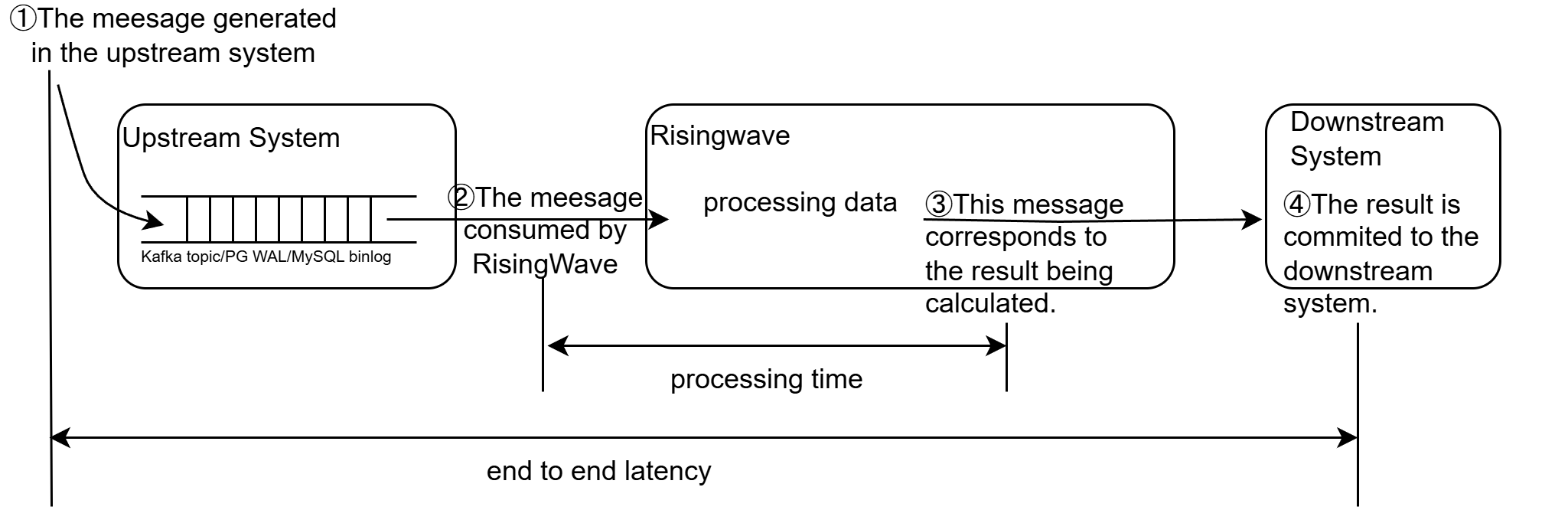
When discussing latency, it’s important to distinguish between end-to-end latency and processing time:- End-to-end latency: The total time it takes from when a piece of data is generated by the upstream system to when the corresponding result is available to the downstream consumer. This includes all processing steps, network delays, and any queuing within RisingWave.
- Processing time: The duration a message spends being actively processed within RisingWave. This is a component of end-to-end latency.
Barrier latency
A barrier is a special type of message that RisingWave injects periodically into the data stream of all sources. Barriers flow along with regular data through the entire stream processing graph (all operators and actors). Barrier latency refers to the time it takes for a batch of barriers (one from each source) to travel from the Meta Node (where they are emitted) to all Compute Nodes (where they are collected). This metric provides a statistical measure of the current processing time within the cluster. See Monitoring and metrics - Barrier monitoring for details on viewing barrier latency.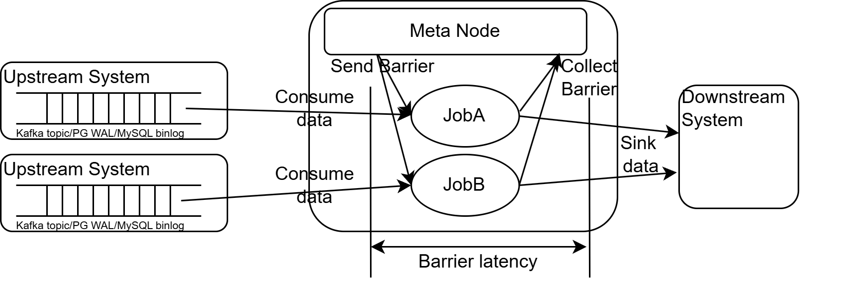
Throughput
Throughput is the number of events (data records) that the system can process in a given amount of time (e.g., rows per second, events per second). For any given RisingWave cluster, the maximum processing throughput is limited by the available resources (CPU, memory, network bandwidth, etc.). See Monitoring and metrics - Data ingestion to check the source throughput. It’s important to understand that the rate at which RisingWave consumes data from the upstream system doesn’t always represent its processing capacity. If the upstream system generates data faster than RisingWave can process it, the data will start to backlog.
Understanding backpressure
How backpressure works in RisingWave
Backpressure occurs when RisingWave’s maximum processing throughput cannot keep up with the upstream system’s data generation rate. In such cases, RisingWave automatically reduces its consumption of upstream data to match its processing capabilities. This prevents data from accumulating excessively within RisingWave, avoiding wasted resources and potential out-of-memory (OOM) errors. Backpressure also helps maintain low and stable processing time and barrier latency.
- Continue to consume data at the maximum rate (200,000 records/second).
- Allow the remaining 800,000 records to backlog in the upstream system.
- Consume and process the backlogged data later, after the traffic spike subsides.
Backpressure propagation between actors
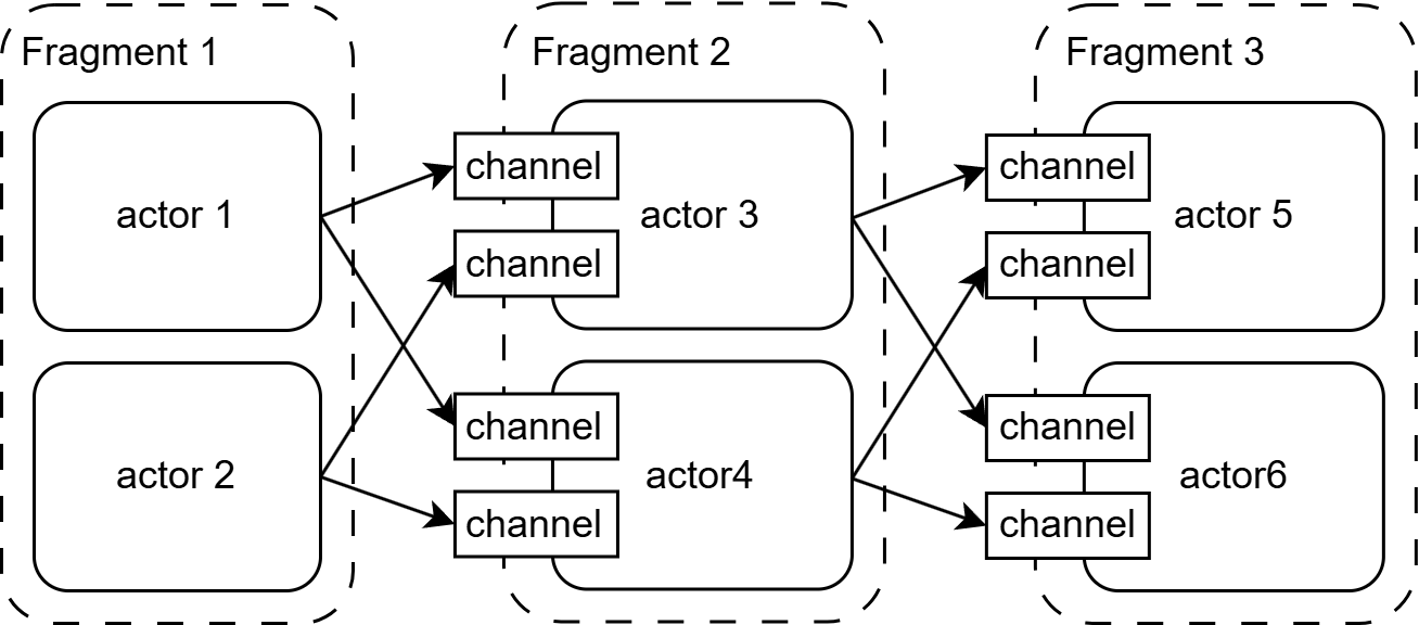
RisingWave’s parallel execution model splits a streaming job into multiple fragments. Each fragment is horizontally partitioned into multiple actors, enabling parallel computation and scalability.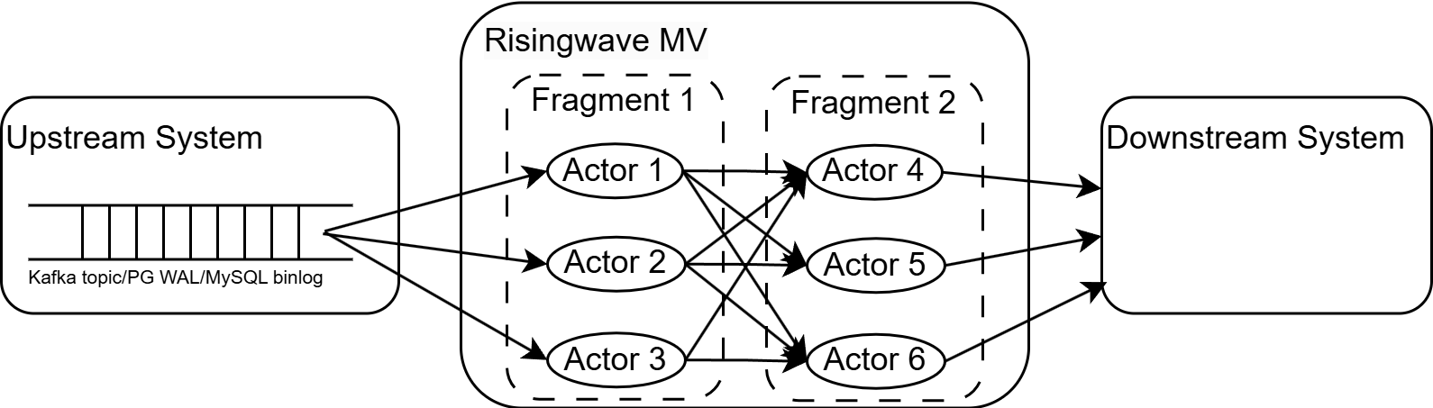
- Consumes data from its upstream channel.
- Processes the data.
- Sends the results to the downstream actor’s channel.
Backpressure details in the source executor
Barriers, as mentioned earlier, are periodically emitted by the Meta Node and sent to a dedicated barrier channel for each source executor. The source executor consumes both barriers (from the barrier channel) and data (from the external system), merging them into a single stream. The source executor always prioritizes the consumption of barriers. It only consumes data from the external system when the barrier channel is empty.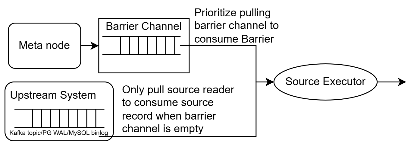
Diagnosing performance issues related to backpressure
Symptoms of backpressure
- High barrier latency: As discussed earlier, high barrier latency is a key indicator of backpressure and slow stream processing.
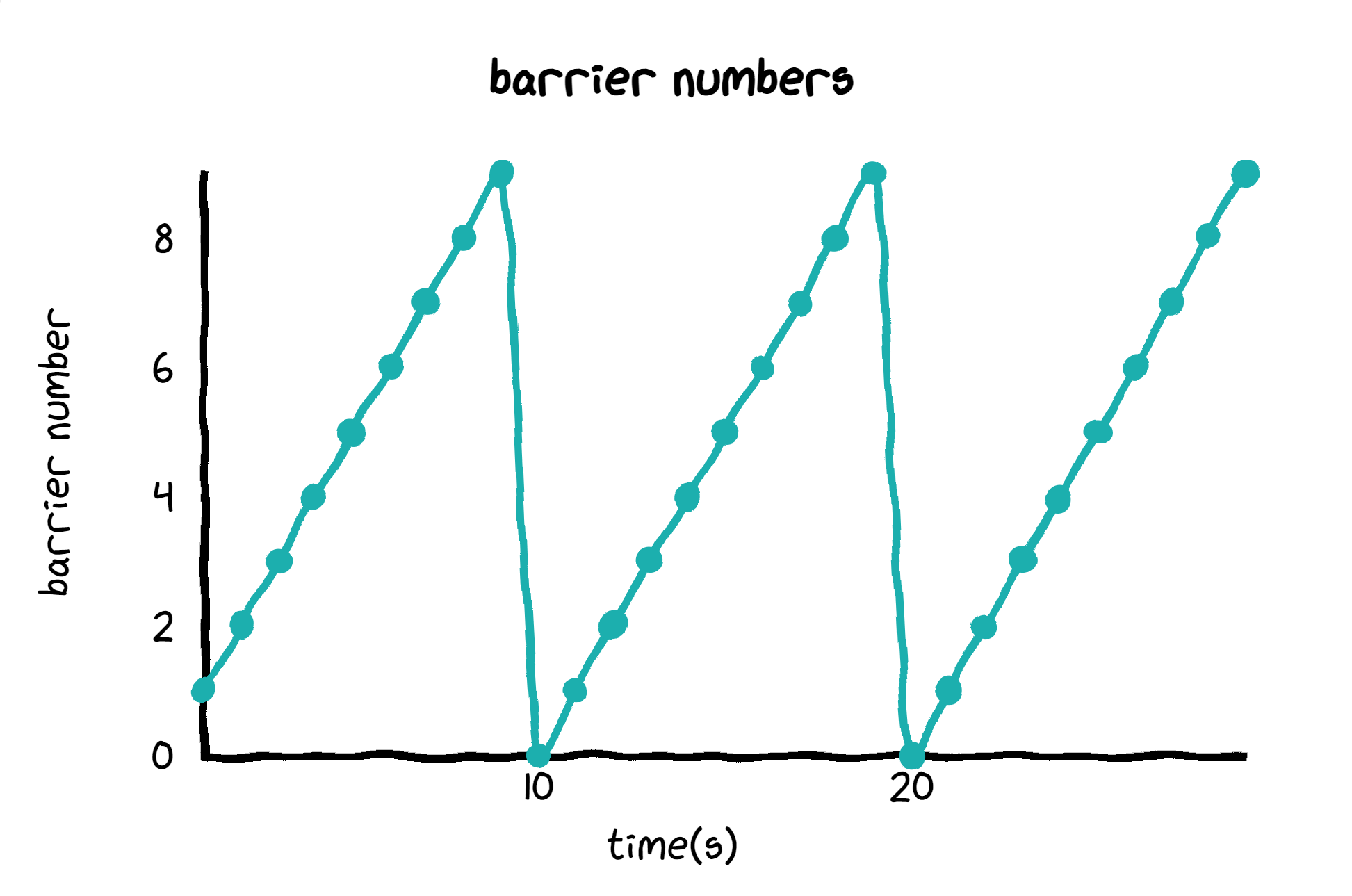
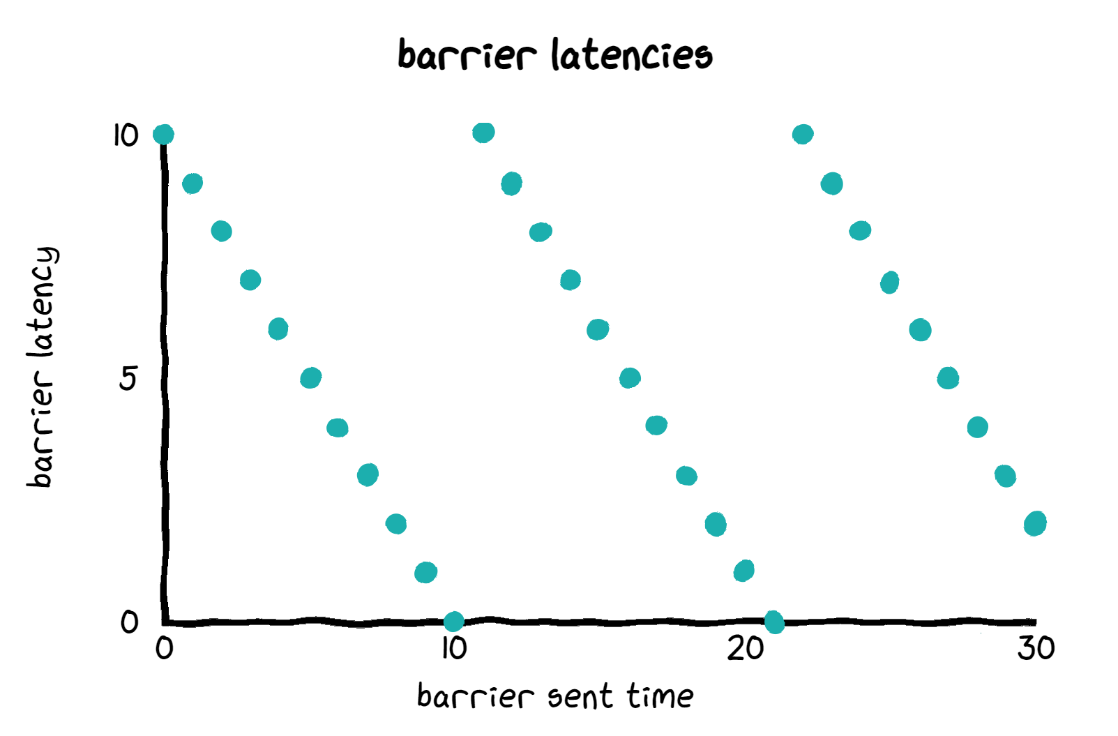
- Sawtooth-like barrier metrics: See the “Backpressure’s Challenges” section below for a detailed explanation of this phenomenon.
- High blocking time ratio between actors.
Identifying bottlenecks
To identify the specific location of a bottleneck causing backpressure:- Use Grafana: Navigate to the “Streaming - Backpressure” panel in the Grafana dashboard.
- Identify High-Backpressure Channels: Look for channels with high “Actor Output Blocking Time Ratio.”
- Find the Frontmost Bottleneck: Backpressure propagates upstream, so the frontmost (closest to the source) actor with high backpressure is likely the root cause.
- Correlate with SQL: Use the RisingWave Dashboard’s “Fragment” panel and the
EXPLAIN CREATE MATERIALIZED VIEW ...command to identify the corresponding part of your SQL query.
Backpressure’s challenges
While backpressure is essential for stability, certain factors can make it less effective or lead to undesirable behavior:The impact of sluggish backpressure on barriers (sawtooth metrics)
Consider a simplified scenario:- No parallelism (single source executor).
- Maximum pipeline throughput: 10,000 rows/second.
- Source executor consumes 100,000 rows before experiencing backpressure.
- Barrier interval: 1 second.
Impact of buffering and solution: limit concurrent barriers in buffer
Buffers between upstream and downstream actors are necessary to smooth out network latency and prevent pipeline stalls. However, excessively large buffers can exacerbate the problems described above. If a downstream channel has a buffer of 100,000, the source might send 100,000 records before experiencing backpressure. In practice, the total buffer size across the entire pipeline can be much larger (the individual buffer size multiplied by parallelism and the number of pipeline layers). This can lead to a situation resembling “batch processing,” with the system alternating between:- Ingesting data at the maximum rate to fill the buffer.
- Entering backpressure and processing the buffered data.
Uncertain consumption per record
Another challenge is that the resource consumption (CPU, memory, I/O) for processing each record can vary significantly. This variability is influenced by factors like:- Data Amplification: Operators like joins can produce multiple output rows for a single input row. The degree of amplification depends on the data itself.
- Cache Thrashing: The performance of stateful operators relies heavily on caching. If data locality is poor (records don’t share common state), cache misses increase, leading to more expensive storage access.