Overview of data processing

It involves applying various operations such as filtering, aggregating, and joining data to derive meaningful information. In the upcoming section, we will delve into the techniques used in the process of transforming and querying data.

​

Declare data processing logic in SQL

RisingWave uses Postgres-compatible SQL as the interface for declaring data processing. We are committed to making it easy to use while being powerful in expression.

Easy to use: By aligning with PostgreSQL’s syntax, functions, and data types, RisingWave eases the learning curve and enhances accessibility for users.Even when creating stream tasks, there is no need to know many concepts related to streaming processing.

Powerful: RisingWave fully supports and optimizes a variety of SQL features, including advanced features such OVER window and different kinds of JOINs. At the same time, we are also committed to expanding the expressive power of SQL, such as by adding semi-structured data types and corresponding expressions.

​

Ad hoc (on read) vs. Streaming (on write)

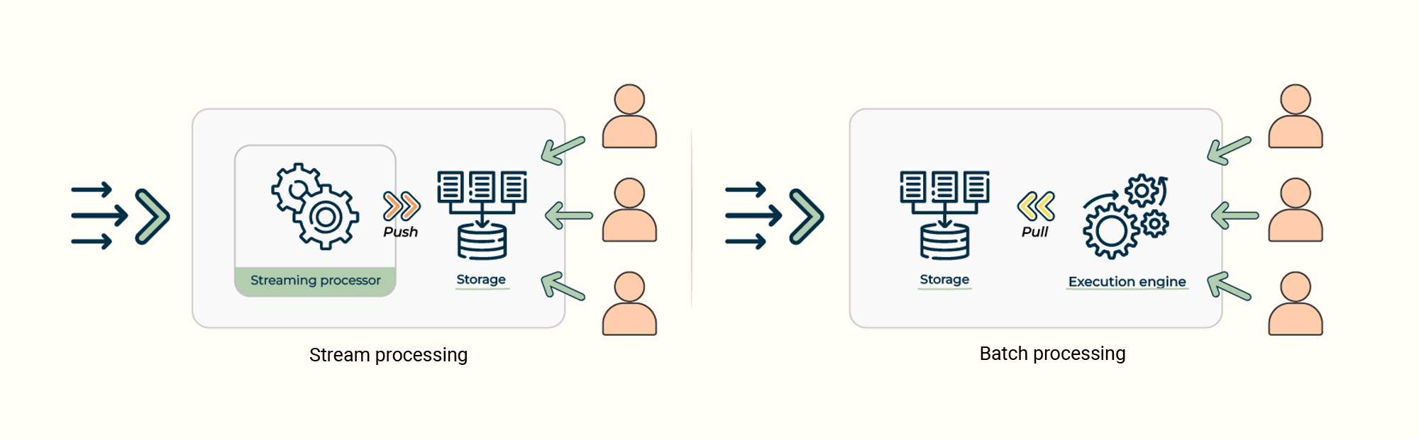
There are 2 execution modes in our system serving different analytics purposes. The results of these two modes are the same and the difference lies in the timing of data processing, whether it occurs at the time of data ingestion(on write) or when the query is executed(on read).

​

Understanding execution modes

Streaming: RisingWave allows users to predefine SQL queries with CREATE MATERIALIZED VIEW statement. RisingWave continuously listens changes in upstream tables (in the FROM clause) and incrementally update the results automatically.

Ad-hoc: Also like traditional databases, RisingWave allows users to send SELECT statement to query the result. At this point, RisingWave reads the data from the current snapshot, processes it, and returns the results.

Both modes have their unique advantages. Here are some considerations:

Cost & Performance: Compared to traditional databases, streaming mode can pre-compute and store results. The heavy lifting is done upfront, eliminating duplicate computation over each ad hoc query, and therefore has better performance and a lower cost.

Flexibility: The streaming mode is less flexible to changes in query requirements. The ad-hoc query usually is created on-the-fly to fulfill immediate and specific information needs. Unlike predefined queries, ad-hoc queries are generated in real-time based on your current requirements. They are commonly used in data analysis, decision-making, and exploratory data tasks, where flexibility and quick access to information are crucial.

​

Querying data across databases

RisingWave supports cross-database queries in both modes, allowing you to access and combine data from multiple databases within your instance for a more comprehensive view. It is implemented through the following key functionalities:

• Enables cross-database binding for batch operations, CREATE MATERIALIZED VIEW, and CREATE SINK.

• Enforces database CONNECT privilege checks for all cross-database queries to ensure secure access.

• Integrates the cross-database snapshot backfill executor, and addresses issues in metadata validation.

• Rejects DROP MATERIALIZED VIEW CASCADE or DROP SINK CASCADE operations with cross-database upstreams to avoid accidental data loss.

• Verifies the existence of log stores for all cross-database upstreams during DDL operations.

To get started, please note the following requirements:

• There must be at least one subscription on the upstream table or materialized view in the external database.

• Users must be a superuser or have CONNECT permissions for the upstream databases, and also have the corresponding QUERY permissions on the relations.

Here is an example demonstrating cross-database queries:

# in database d1
CREATE TABLE t1 (v1 INT);

# at lease one subscription required to enable log store for t1
CREATE subscription sub FROM t1 WITH (retention = '1D');

# switch to database d2
SET DATABASE TO d2;

CREATE TABLE t2 (v2 INT);

SELECT COUNT(*) FROM d1.public.t1;

CREATE MATERIALIZED VIEW mv1 AS SELECT * FROM d1.public.t1;

CREATE MATERIALIZED VIEW mv2 AS SELECT t1.v1, t2.v2 FROM d1.public.t1 JOIN t2 ON t1.v1 = t2.v2;

​

Examples

​

Create a table

To illustrate, let’s consider a hypothetical scenario where we have a table called sales_data. This table stores information about product IDs (product_id) and their corresponding sales amounts (sales_amount).

product_id | sales_amount
------------+--------------
          1 |           75
          2 |          150
          2 |          125
          1 |          100
          3 |          200

You can use the following statement to create this table.

CREATE TABLE sales_data (
    product_id INT,
    sales_amount INT
);

INSERT INTO sales_data (product_id, sales_amount)
VALUES
    (1, 100),
    (1, 75),
    (2, 150),
    (2, 125),
    (3, 200);

​

Create a materialized view to build continuous streaming pipeline

Based on the sales_data table, we can create a materialized view called mv_sales_summary to calculate the total sales amount for each product.

CREATE MATERIALIZED VIEW mv_sales_summary AS
SELECT product_id, SUM(sales_amount) AS total_sales
FROM sales_data
GROUP BY product_id;

By the SQL statement above, you have successfully transformed the data from the sales_data table into a materialized view called mv_sales_summary. This materialized view provides the total sales amount for each product. Utilizing materialized views allows for precomputing and storing aggregated data, which in turn improves query performance and simplifies data analysis tasks.

​

Ad-hoc query on materialized view’s result

Then we can directly query the materialized view to retrieve the transformed data:

SELECT * FROM mv_sales_summary;

----RESULT
 product_id | total_sales
------------+-------------
          1 |         175
          2 |         275
          3 |         200
(3 rows)

Also, analysts or applications can send more flexible and complex ad-hoc queries, such as querying how many products have higher sales volumes than a specific product

SELECT count(*) FROM mv_sales_summary where mv_sales_summary.total_sales >
    (SELECT total_sales FROM mv_sales_summary where product_id = 1);

----RESULT
 count
-------
     2
(1 row)